​​Prototyping and Benchmarking Machine Learning-Based Digital Predistortion with the NI RF Hardware​

​Because of the huge advancements in the area of artificial intelligence (AI) and machine learning (ML) within recent years, there are new ways for solving challenging problems in many industries. In the wireless domain, the use of AI/ML is one of the most promising technology candidates which is currently being discussed to provide new services and improve mobile networks.¹ Among others, AI/ML can help mobile network operators (MNOs) to improve the efficiency of their networks and drive operating costs down, one of the MNOs’ major goals. These improvements could mean a more efficient use of spectrum through smarter allocation of resources in the time, frequency, and spatial domain—or better interference compensation schemes. Furthermore, the use of AI/ML could also enable energy efficiency improvements to address one of the main cost drivers for base stations. For example, smarter ways to switch on and off base stations on a per-need basis could create more efficient usage of power amplifiers.  

​While AI/ML is already being used successfully at the network level, significantly more challenges exist for using AI/ML at the lower layers, such as the RF layer, physical layer (PHY), or MAC layer. The tight timing constraints at these lower layers mean it is more difficult to develop and deploy robust and reliable AI/ML-based algorithms that provide significant gains over traditional methods.² Therefore, this area is still in its research phase to understand the different trade-offs to successfully use AI/ML in areas where it makes sense and to prove that those AI/ML algorithms are robust and reliable in real network deployments. Ultimately, one must prove that the use of AI/ML shows clear advantages against traditional approaches to justify new investments.  

​Today’s AI/ML research activities on RF/PHY/MAC layers of wireless communications systems include the following popular areas:  

• ​RF—ML-based digital predistortion (DPD) to improve the efficiency of power amplifiers and save energy.
• PHY—ML-based channel estimation and symbol detection to improve spectrum efficiency by using fewer or no pilot symbols as well as to improve energy efficiency by having the same transmission quality at a lower signal-to-noise ratio.
• ​MAC—ML-based beam management to improve beam acquisition and tracking with the goal to steer energy of an antenna array in the direction of a user. With that, the spectrum can be utilized more efficiently by serving more users in a cell. Furthermore, energy can be saved to adapt signal-to-noise ratio at the receiver to the actual quality of service needs.

​In another NI white paper, we described a framework to prototype and benchmark a real-time neural receiver utilizing NI SDR devices. In this white paper, we describe a case study of how to prototype and benchmark ML algorithms for digital predistortion of power amplifiers using NI RF hardware. We provide a short overview of some typical neural networks that have been researched for DPD. We also describe how we implemented a prototype application for training an ML-DPD model with waveform data from an actual PA, validating its predistortion performance with the PA and benchmarking the performance against other state-of-the-art algorithms. At the end, we provide key learnings from our experimentation work and summarize challenges and research questions for using ML-based DPD in practical deployments.

​It is well known that power amplifiers (PAs) are most efficient when they operate in their nonlinear region. Unfortunately, in this region the PA generates unwanted out-of-band emissions from intermodulation caused by nonlinear characteristics of the PA. Digital predistortion is usually applied to the transmitter waveform to compensate for the distortions. The compensation, or the predistortion, applies the inverse of the nonlinearity of a PA in digital baseband, so that the combined response of DPD and the PA is again linear. Figure 1 illustrates this compensation scheme. As a result, DPD enables a PA to operate in a nonlinear region at higher power efficiency without losing linearity.  

​Ever-demanding data rates require more bandwidth that is specifically available at higher carrier frequencies that usually require antenna arrays to steer the energy and overcome the high path loss. Specifically for PAs designed to operate under these conditions DPD becomes more and more challenging because of the following reasons:

• ​Non-static behavior of PAs where the underlying model changes for dynamic operation conditions  
• ​Increased complexity of PA non-linearities where the Volterra-series based models are no longer suitable  

​To address the previously mentioned challenges for modern communication systems, innovative approaches are needed for DPD. Machine learning is one approach that is being actively researched by industry and academia, that we will describe in the following section.

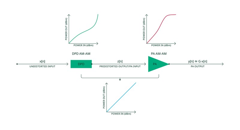
Figure 1. Principle of Digital Predistortion

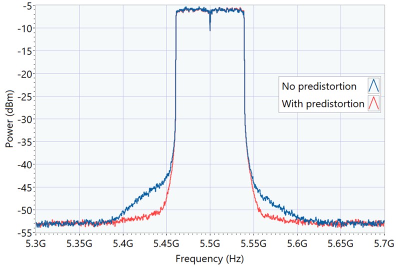
Figure 2. Spectral Leakage Improvement Due to DPD

​Figure 2 shows an example of improvement in the spectral leakage from predistortion by comparing the output signal of a Wi-Fi PA with and without applying digital predistortion. The main challenge for DPD is estimating the nonlinearity of the used PA, which means estimating the underlying PA model. Traditionally, for memoryless nonlinearities, the approach of static lookup tables based on measured AM/AM and AM/PM distortions has been used. To deal with non-linearities with memory, Volterra-series based models such as memory polynomial model (MPM) and generalized memory polynomial (GMP) model are typically used.

​Neural networks have been researched for use in behavioral modeling and digital predistortion because of their ability to model nonlinear systems, like a power amplifier having nonlinear behavior with nonlinear memory effects.

​A couple of decades ago, a team proposed⁵ a real-valued time-delay neural network (RVTDNN) model based on a multilayered perceptron (MLP) structure for behavioral modeling of 3G power amplifiers. It used tapped delay lines on in-phase (I) and quadraturephase (Q) components of the signal to model short-term memory effects of the PA. A fully recurrent neural network (FRNN) was proposed6 for behavioral modeling of PAs for 3G cellular communication systems with strong memory effects along with high nonlinearity. It uses complex signals as input with weights and biases being complex. Digital predistortion of power amplifiers using neural networks was extensively investigated and validated for WCDMA signals,⁷ which proposed a real-valued focused time-delay neural network (RVFTDNN), which avoids computation of complex gradients.  

​Recurrent neural networks (RNNs) have the inherent ability to model memory effects—the situation where the current output depends on not just the current input but also on past inputs. However, RNNs have challenges capturing long-term memory effects caused by the issue of vanishing gradients. Long short-term memory (LSTM) networks were proposed to deal with the issue of vanishing gradients in RNNs.⁸

​LSTM networks employ different types of gates to better control to what extent past and new information impact the network memory states.⁹ For behavioral modeling of GaN PAs with long-term memory effects, a team studied10 use of LSTM networks to work around the limitation of FRNN.⁷ Other enhanced or optimized versions of RNN-based networks such as bidirectional LSTM (BiLSTM) and gated recurrent unit (GRU) networks are described for the purpose of digital predistortion^11,12 and references therein. Recently, convolutional neural networks (CNNs) were explored for behavioral modeling and predistortion of PAs.¹³  

​Neural networks have also been proposed to avoid continuous parameter update of digital predistortion in massive MIMO systems with active antenna arrays, which suffer from beam-dependent load modulation.¹⁴ For this case study, we chose to implement an LSTM-based neural network for DPD.  

​Figure 3 shows all layers of the implemented neural network. The network gets samples of the undistorted complex time-domain signal x[n] as input and provides samples for the predistorted complex time-domain signal z[n] at the output. At one timestep, the input to the LSTM layer are in-phase and quadrature-phase components i, q of the current and the past M input signal samples, where M is the memory depth.  

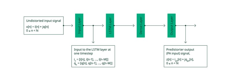
Figure 3. Model Architecture

​The neural network must be taught the target DPD functionality using a training data set during the learning (training) stage. Common learning architectures for a DPD model could be a direct learning architecture (DLA), an indirect learning architecture (ILA), or an iterative learning control (ILC)-based architecture. For our case study, we chose ILC as the source for training data as it provides an optimal PA predistorted input signal that linearizes the PA.  

​ILC-based DPD is useful as a benchmark for evaluating the performance of any DPD scheme.  

​Figure 4 shows the learning architecture for ILC to iteratively compute a predistorter output signal, z[n], which is also the input signal to the PA, given an undistorted input signal, x[n]. After enough iterations, the final computed predistorter output signal can be assumed to be the ideal predistorter output signal and ideal PA input signal, zideal [n]

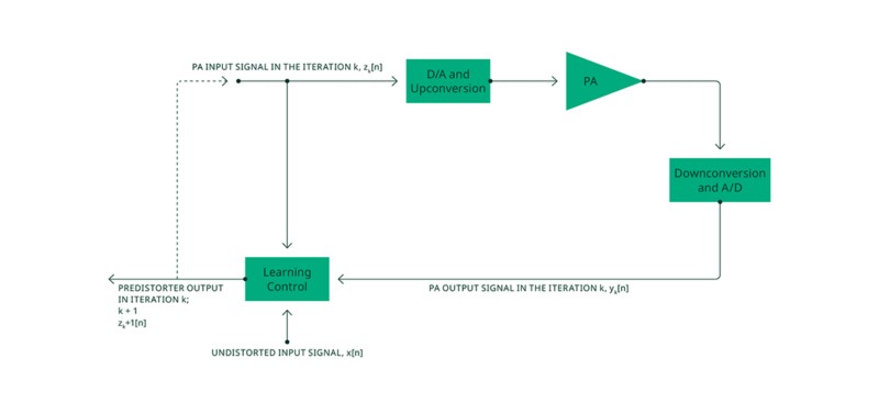
Figure 4. Learning Architecture: Iterative Learning Control

​One or more pairs of an undistorted input signal and its corresponding ideal predistorter output signal can be used to train or fit parameters of any DPD model, including traditional generalized memory polynomial models—or as in our case, a neural network model. During the training process, the ideal predistorter output signal(s) acts as ground truth for target output signal(s) the DPD model should learn to generate for the respective undistorted input signal(s). This process is shown in Figure 5.

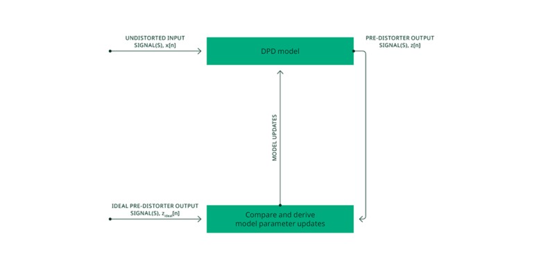
Figure 5. DPD Model Training

​We created a prototype application to study the entire workflow of a machine-learning-based DPD implementation.

​The application runs on a PXI controller in an NI PXI chassis using an NI PXI Vector Signal Transceiver (VST) to generate and analyze RF signals and an NI PXI Source Measure Unit to provide DC power and drive digital control lines to the PA. A block diagram of the test setup used is shown in Figure 6.  

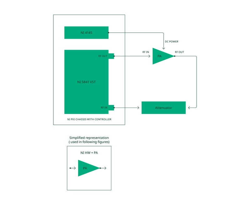
Figure 6. Test Setup Showing Hardware Connections

​The application is used to perform these steps:  

1. ​Create waveform data to be used for training and testing.  
2. Create a training data set using an actual PA.  
3. Use the training data set to train a neural network model.  
4. Deploy the trained neural network model to pre-distort the input to an actual PA.  

​Figure 7 shows these user actions. The subsequent sections explain these in detail. Except for the neural network model training, the application is written in NI LabVIEW. It uses the NI RFmx software for performing standard RF measurements on the PA using an NI Vector Signal Transceiver (VST). It uses NI RFmx Waveform Creator to create waveform files. Neural network model training is implemented in Python using TensorFlow and Keras libraries. For faster execution, the training is run on a Linux server with an NVIDIA GPU.

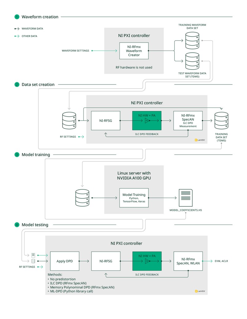
Figure 7. ML-DPD Prototype Application User Actions

​Step 1: Create Waveform Data NI-RFmx Waveform  

​Creator can be used to create waveforms compliant to a communication standard. For our case study, we used NI-RFmx Waveform Creator for WLAN to create waveform data for multiple 802.11ax frames of 1 ms length with a channel bandwidth of 80 MHz. For the payload data, we used different pseudorandom data bit sequences and varied the modulation orders from BPSK to 1024-QAM. The waveforms are stored in a TDMS file format.  

​These waveforms form the undistorted input signals in our data sets. Based on user-specified inputs, the waveform data set is split into a) a training waveform data set and b) a test waveform data set. For example, our training waveform data set typically contained some of the BPSK waveforms.  

​Step 2: Create a Training Data Set Using an Actual PA  

​The next step is to create a training data set. To train the NN model, we need the undistorted input signal and its corresponding ideal predistorter output signal, computed using an actual PA at a predecided set of operating conditions of the PA, like the RF center frequency and input average power level.  

​For each of the undistorted input signals read from waveform TDMS files and PA operating conditions, this is how the ideal predistorter output signal is computed: RF settings are configured on NI-RFSG according to the desired PA operating condition. NI-RFSG generates an RF signal, read from a waveform TDMS file from the training waveform data set created in Step 1, at the input of the PA using the vector signal generator within an NI VST. The output signal of the PA is acquired by the vector signal analyzer within an NI VST and measured using the IDPD (ILC DPD) measurement of NI-RFmx SpecAn. The measurement returns a predistorted waveform, which we record as the ideal predistorter output signal.  

​The waveform I/Q data along with the associated metadata of signal and RF settings are recorded in a training data set file of a TDMS format.  

​The training data set file contains the following information:  

• ​I/Q waveform data  
  • ​Undistorted input signal—an unimpaired baseband signal, which in our case is an 802.11ax waveform created in Step 1. It is possible to use other waveforms like a multitone signal or a waveform compliant to any wireless communication standard
• ​Ideal predistorter output signal—the waveform computed using iterative learning control (ILC). For this, we used the ILC-based DPD (IDPD) measurement in NI-RFmx SpecAn.  
• ​Metadata (important contents with example values)
  • ​ Waveform configuration examples  
    • ​Standard: 802.11ax  
    • ​Bandwidth: 80 MHz  
    • ​Modulation order: BPSK  
    • ​Waveform length: 1 ms  
    • ​Waveform PAPR: 10.8 dB  
• ​RF settings examples  
  • ​RF center frequency: 5.5 GHz  
  • ​PA input average power level: -10 dBm  

​As mentioned earlier, a researcher could use this data set to train any model for the predistorter. The process of acquiring the training data set need not be repeated unless there is a change in training conditions

​Step 3: Train a Model

​After we have a training data set, the next step is to train the model. The process used is shown in Figure 8. The training application is written in Python using TensorFlow and Keras libraries and is run on a Linux server with an NVIDIA A100 GPU for faster training speeds. The training waveforms data set is first divided into training, validation, and test data sets. During training, the model is fed the undistorted input signals from the training and validation data sets, and it predicts the respective predistorter output signals.  

​The latter are compared to the related ideal predistorter output signals, the respective training and validation loss is calculated. The training loss is used to update the model coefficients. The validation loss is monitored to evaluate whether the model generalizes well and to detect overfitting. The loss metric we use is the mean squared error (MSE) between the predicted and the ideal desired model output (the ideal predistorter output).

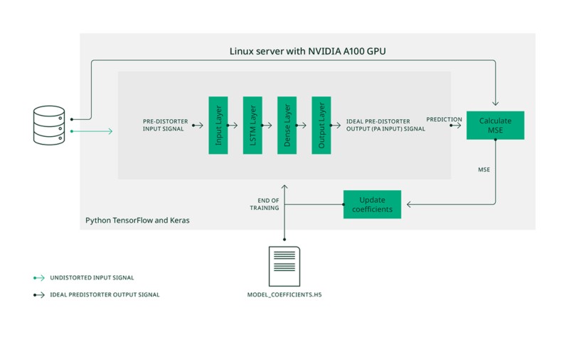
Figure 8. Model Training

​During our training and validation experiments we observed that training was successful when we reached MSE loss values below 10^-4 and the training and validation loss curves smoothly converge towards a similarly low value, as shown in Figure 9. The final output of the training process is an H5 file containing the coefficients of the trained model.  

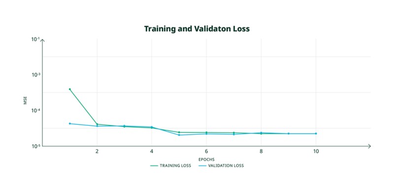
Figure 9. Desired Training and Validation Loss Curves

​Step 4: Deploy the Model to Predistort the Input to an Actual PA

​The trained ML-DPD model must be tested to verify it can also work for waveform data the model has not been trained on. For this, the trained model is used to apply DPD on the waveform data from the test waveform data set before generating a signal into the PA. The model is applied using a Python library call from LabVIEW by passing in the model coefficients file and the waveform data as inputs. Its performance is compared against ILC DPD. Along with ILC DPD and ML-DPD, the testing application can also apply conventional DPD methods, like memory polynomial DPD to benchmark performance of ML-DPD against them. The performance can be compared in terms of standard metrics like RMS EVM and ACLR using NI RFmx SpecAn and RFmx NR or RFmx WLAN (based on the signal type).

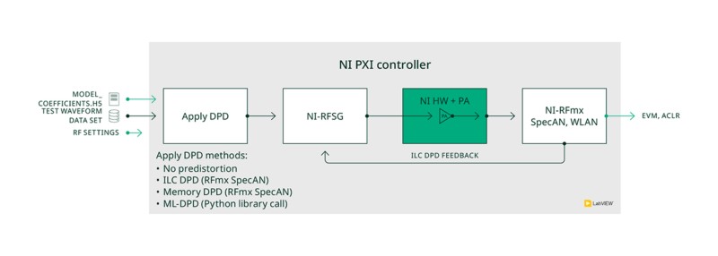
Figure 10. Desired Training and Validation Loss Curves

​The prototype application was used to design and test ML-DPD for a TriQuint Wi-Fi PA (evaluation board: TQP887051).

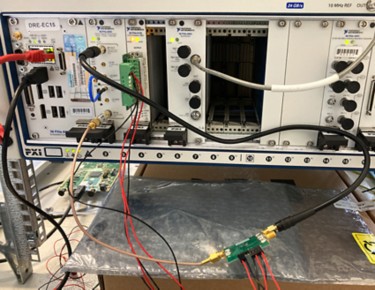
Figure 11. Test Setup for ML-DPD Prototype Application with a PXI System (Left) and a TriQuint Wi-Fi PA (Right)

​For testing, we selected the center frequency of 5.5 GHz and the PA input average power level of -8.5 dBm. AM-AM characteristics of the PA at this operating point were measured using NI-RFmx SpecAn on an 802.11ax, 80 MHz, 1024-QAM waveform of approximately PAPR 10.5 dB is shown in Figure 11. The PA shows a linear gain of around 25.7 dB. At the peak input power level of around 2 dBm, the PA’s output shows gain compression of around 3 dB.

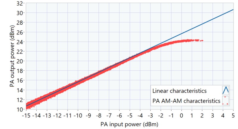
Figure 12. AM-AM characteristics of the PA at 5.5 GHz and input average power level of -8.5 dBm.

​We trained the model at this operating point with a training data set that contained thirteen different 802.11ax frames with BPSK modulation scheme. The model parameter memory depth was set to four samples, resulting in a model size of around 24,000 parameters. The validation data set contained three 802.11ax frames with BPSK modulation scheme. Each 802.11ax frame is of 1 ms length. Figure 12 shows the loss curves observed during the training. The observed training and validation losses of around 2×10^-4 are acceptable. We tried different values for memory depth and the value of four was found to be suitable.

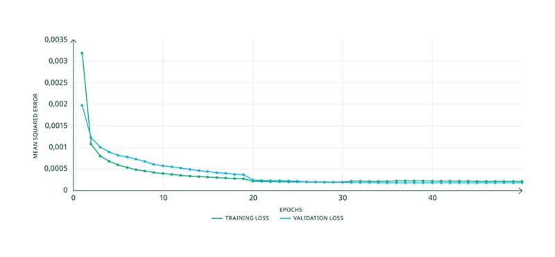
Figure 13. Loss Curves for the Model Trained

​We then tested the model with different waveform data and at different input average power levels ranging from -15 dBm to -8.5 dBm in steps of 0.25 dB. For the example test result in Figure 13, we used a 1024-QAM waveform data file from the test data set. This is the same waveform which was used for measuring AM-AM characteristics shown above. We measured RMS EVM using NI-RFmx WLAN for three modes of predistortion:  

1. No predistortion  
2. ILC DPD  
3. ML-DPD  

​We compared the ML-DPD performance with that of ILC DPD, because ML-DPD was trained with ILC DPD data acting as ground truth. As seen in the graph, both ILC DPD and ML-DPD show significant improvement in EVM as compared to EVM measured without any predistortion. For the input power level of -8.5 dB, which was used during training, the trained ML-DPD provides the same EVM performance as the optimal ILC DPD.  

​For the majority of other input power levels, the ML-DPD EVM performance is close (within 1 dB) to the values reached with ILC DPD. Only for the input power range from -10.5 dBm to -9.5 dBm, we see a slightly stronger EVM deviation of up to 2 dB between ML-DPD and the optimal ILC DPD, which potentially could be further reduced by incorporating additional training data from these power levels into the training process.

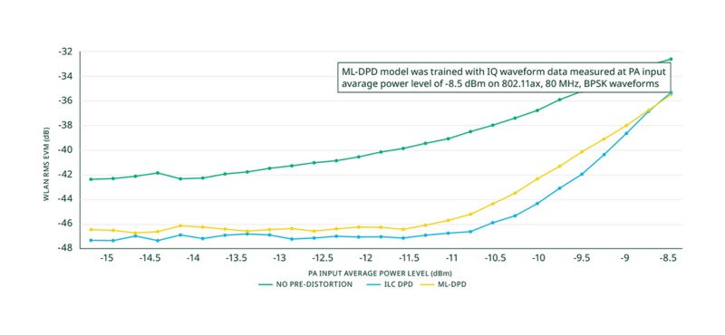
Figure 14. WLAN RMS EVM with and without predistortion.

​In this paper, we showed how NI software and hardware can be used to prototype, validate, and benchmark the use of machine learning approaches for digital predistortion of power amplifiers. We used the same prototyping system for creating training data and validating inference performance against other state-ofthe-art DPD algorithms. We showed an example result for applying an LSTM-based neural network for the DPD of a Wi-Fi PA. The results show that for this specific example, the performance of the ML DPD is close to the lower bound given by ILC DPD that we used as reference for the ML model training.  

​It is worth noting that while this example’s result looks good, during our studies we also found situations where our example ML DPD model did not perform as expected. One key learning of our investigation is that it is always important to compare and benchmark new ML DPD models against other DPD approaches to better understand the trade-offs between efficiency and complexity. It is important to prove on realistic systems where the use of ML DPD can lead to benefits and where traditional DPD algorithms are better suited.  

​We believe the following research areas need more research and innovation:  

• ​Trade-offs between bigger generalized ML DPD models versus smaller models that get retrained and adapted during operation and the corresponding training strategies.  
• ​Performance-optimized, real-time capable, low complexity ML DPD models for FPGA, GPU, or CPU-based target platforms.  
• ​Low power consumption of the ML DPD algorithm on the digital processing platform so that DPD does not reduce power savings of the PA.  
• ​Intelligent validation and test methodologies to efficiently prove reliability and robustness of the data-driven ML DPD models.  

​To investigate those research questions, the described NI RF hardware with its leading-edge hardware and software can help you understand the specific tradeoffs of ML DPD that have to be considered for the design of more energy-efficient RF systems. This consideraton will ultimately also lead to more trust in using advanced AI technologies in such critical systems like mobile communication networks.

​1 Sundarum, Meesha. “3GPP Technology Trends.” 5G Americas, 2024. https://www.5gamericas.org/3gp-technology-trends.  

​2 Polese, M., Dohler, M., Dressler, F., Erol-Kantarci, M., Jana, R., Knopp, R., Melodia, T., “Empowering the 6G Cellular Architecture with Open RAN.” IEEE Journal on Selected Areas in Communications, November 2023.  

​3 Summerfield, Steve. “How to Make a Digital Predistortion Solution Practical and Relevant.” Microwaves & RF, 2022. https://www.mwrf.com/technologies/embedded/systems/article/21215159/analog-devices-how-to-make-adigital-predistortion-solution-practical-and-relevant.

​4 Zhu, Anding, January 10, 2023. “Digital Predistortion of Wireless Transmitters Using Machine Learning.” IEEE MTT-S Webinar.

​5 Liu, T., Boumaiza, S., and Ghannouchi, F. M., March 2004. “Dynamic Behavioral Modeling of 3G Power Amplifiers Using Real-Valued Time-Delay Neural Networks.” IEEE Transactions on Microwave Theory and Techniques, 52 (3): 1025–1033.  

​6 Luongvinh, Danh and Kwon, Youngwoo, 2005. “Behavioral Modeling of Power Amplifiers Using Fully Recurrent Neural Networks.” IEEE MTT-S International Microwave Symposium Digest: 1979–1982.  

​7 Rawat, M., Rawat, K., and Ghannouchi, F. M., January 2010. “Adaptive Digital Predistortion of Wireless Power Amplifiers/Transmitters Using Dynamic Real-Valued Focused Time-Delay Line Neural Networks.” IEEE Transactions on Microwave Theory and Techniques 58 (1): 95-104.

​8 Hochreiter, S and Schmidhuber, J., November 1997. “Long short-term memory.” Neural Computation 9 (8): 1735–1780.  

​9 Olah, Christopher, “Understanding LSTM Networks.” Understanding LSTM Networks -- colah’s blog, August 27, 2015. https://colah.github.io/posts/2015-08-Understanding-LSTMs/.  

​10 Chen, P., Alsahali, S., Alt, A., Lees, J., and Tasker, P. J., 2018. “Behavioral Modeling of GaN Power Amplifiers Using Long Short-Term Memory Networks.” 2018 International Workshop on Integrated Nonlinear Microwave and MillimetreWave Circuits (INMMIC), Brive La Gaillarde, France, 2018, pp. 1–3.  

​11 Li, G., Zhang, Y., Li, H., Qiao, W., and Liu, F., 2020. “Instant Gated Recurrent Neural Network Behavioral Model for Digital Predistortion of RF Power Amplifiers.” IEEE Access, vol. 8: 67474–67483.  

​12 Kobal, T., Li, Y., Wang, X., and Zhu, A, June 2022. “Digital Predistortion of RF Power Amplifiers with Phase-Gated Recurrent Neural Networks,” IEEE Transactions on Microwave Theory and Techniques 70 (6): 3291–3299.

​13 Hu, X, et al., August 2022. “Convolutional Neural Network for Behavioral Modeling and Predistortion of Wideband Power Amplifiers.” IEEE Transactions on Neural Networks and Learning Systems 33 (8): 3923–3937.  

​14 Brihuega, A., Anttila, L, and Valkama, M. August 2020. “Neural-Network-Based Digital Predistortion for Active Antenna Arrays Under Load Modulation.” IEEE Microwave and Wireless Components Letters 30 (8): 843–846​

• Learn more about the NI VST
• Explore the RF measurement library
• Discover how AI is used in wireless systems
• Learn more about GPU integration with LabVIEW and NI PXI hardware